
Contrastive learning의 대표적 알고리즘 중 하나인 SimCLR에 대해서 알아보자. 교수님의 말씀에 따르면 내가 이 강의를 들을 당시 2~3년 전 연구자들, 지금으로 따지면 4~5년 전의 이미지 쪽 건드리는 연구자들에게는 필수였던 방법론이었다고 한다. 얘도 마찬가지로 positive pair는 당기고, negative pair는 미는 방식이다. 그럼 어떤 식으로 돌아가는 건지 본격적으로 알아보자. 참고로 저자들 중에 최근 노벨상 수상하신 Geoffrey Hinton이 있다.
원문링크: https://arxiv.org/abs/2002.05709
A Simple Framework for Contrastive Learning of Visual Representations
This paper presents SimCLR: a simple framework for contrastive learning of visual representations. We simplify recently proposed contrastive self-supervised learning algorithms without requiring specialized architectures or a memory bank. In order to under
arxiv.org
Contrastive Learning이 잘 작동하기 위해서는 뭐가 필요할까?
저자들은 시작하기 전 contrastive learning framework가 잘 작동하려면 어떤 요소들이 필요한 지에 대한 분석을 했는데, 한 번 보자.
- Strong, compositional augmentations
– crop, color-jitter, Gaussian blur 등 다양한 augmentation을 조합해 hard positive를 생성해야 한다. - Nonlinear projection head
– encoder 위에 소형 MLP projection head를 두고, contrastive loss를 이 출력 에만 적용한다. - ℓ₂-normalization + temperature
– projection된 embedding을 ℓ₂-normalize하고, softmax의 temperature를 적절히 조정해야 학습이 안정되고 신호가 sharpen된다. - Large batch size, long training, high-capacity networks
– 충분한 수의 negatives를 확보할 수 있는 큰 batch, 긴 학습 스케줄, 그리고 깊거나 넓은(backbone) 네트워크가 필요하다.
그래서 SimCLR은 위의 요소들을 다 포함한 framwork가 될 것이며, 위에걸 다 적용한 결과 ImageNet ILSVRC-2012에서 76.5%, 1%의 ImageNet label을 활용해 fine-tuning한 결과 85.8%로 SOTA를 달성했다고 한다.
SimCLR Method
SimCLR의 method를 step-by-step으로 알아볼 것이다. 과정을 figure로 보자.
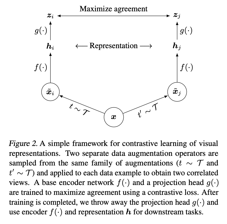
1. Data Augmentation
위의 사진을 보자. x가 하나의 원본 이미지이다. 여기서 두 개의 augmented image가 각각 나온다. x_i 와 x_j가 나온다. 이 두 개는 어떻게 나오느냐 하면, 두 개가 동일한 여러 단계의 data augmentation method를 거치는데, 이때 augmentation의 parameter를 각각 independently sampling 해서 각각 다른 두 개의 augmented image를 만든다.
여러 단계의 data augmentation method는,
1. Random Image Crop
2. Random Color Distortion
3. Gaussian Blur

이렇게이다. 그리고 이렇게 나온 i와 j는 "positive pair" 로 분류할 것이다. 이후 ablation study에서 저자들은 crop과 color distortion이 더 중요하고, blur은 extra boost 정도라고 말한다.

2. Encoder Network f(⋅)
SimCLR에서 사용하는 encoder는 standard한 ResNet50이긴 한데, 마지막에 classifier head를 뺀 구조이다.

3. Projection Head g(⋅)
2번을 거치면 representation인 h가 나오는데, h 위에 small MLP head를 쌓아줄 것이다.

이게 왜 있냐면, encoder에서 나온 image representation h에 바로 contrastive loss를 적용하는게 아니라, z=g(h)인 z를 가지고 constrastive loss를 계산해볼 것이다.
이렇게 하는 이유는, 좀 더 "순수한" h를 가지기 위함이다. 이 MLP head가 없으면 우리의 image representation h는,
1. 이따가 적용할 InfoNCE loss의 복잡한 구조인 유사한건 당기고 다른건 미는 걸 만족하는 동시에,
2. 우리가 최종적으로 진짜 하고 싶은 classification 같은 downstream task에 적합한 representation vector가 되어야 한다.
h는 이걸 전부 만족하도록 훈련되어야하는 것이다.
근데 여기서 희생양이 될 g를 introduce하는 순간, 우리의 h는 InfoNCE에 대해서 걱정하지 않아도 된다. g를 적용한 후의 결과에다가 InfoNCE loss를 적용할 것이기 때문이다. 그리고 g는 MLP layer 이므로 non-linear한 걸 배울 수 있는데, 이런 non-linear 한 요소들이 더 추가된 결과물로 InfoNCE loss를 적용할 것이기 때문에 뭐가 유사한 사진들인지, 뭐가 다른 사진들인지에 대한 정보를 더 많이 가지고 있어, InfoNCE가 더 잘 먹힐 수 있다.

4. Normalization
ℓ₂-normalize 해주고,
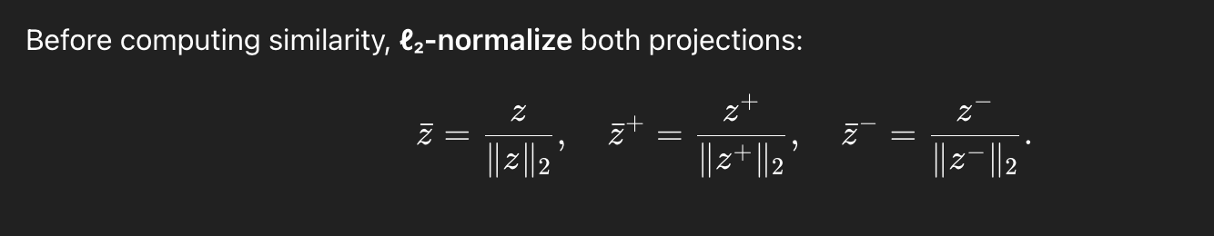
5. Contrastive Loss
distance를 계산해 준 다음에 minibatch 당 contrastive loss를 계산해주자.
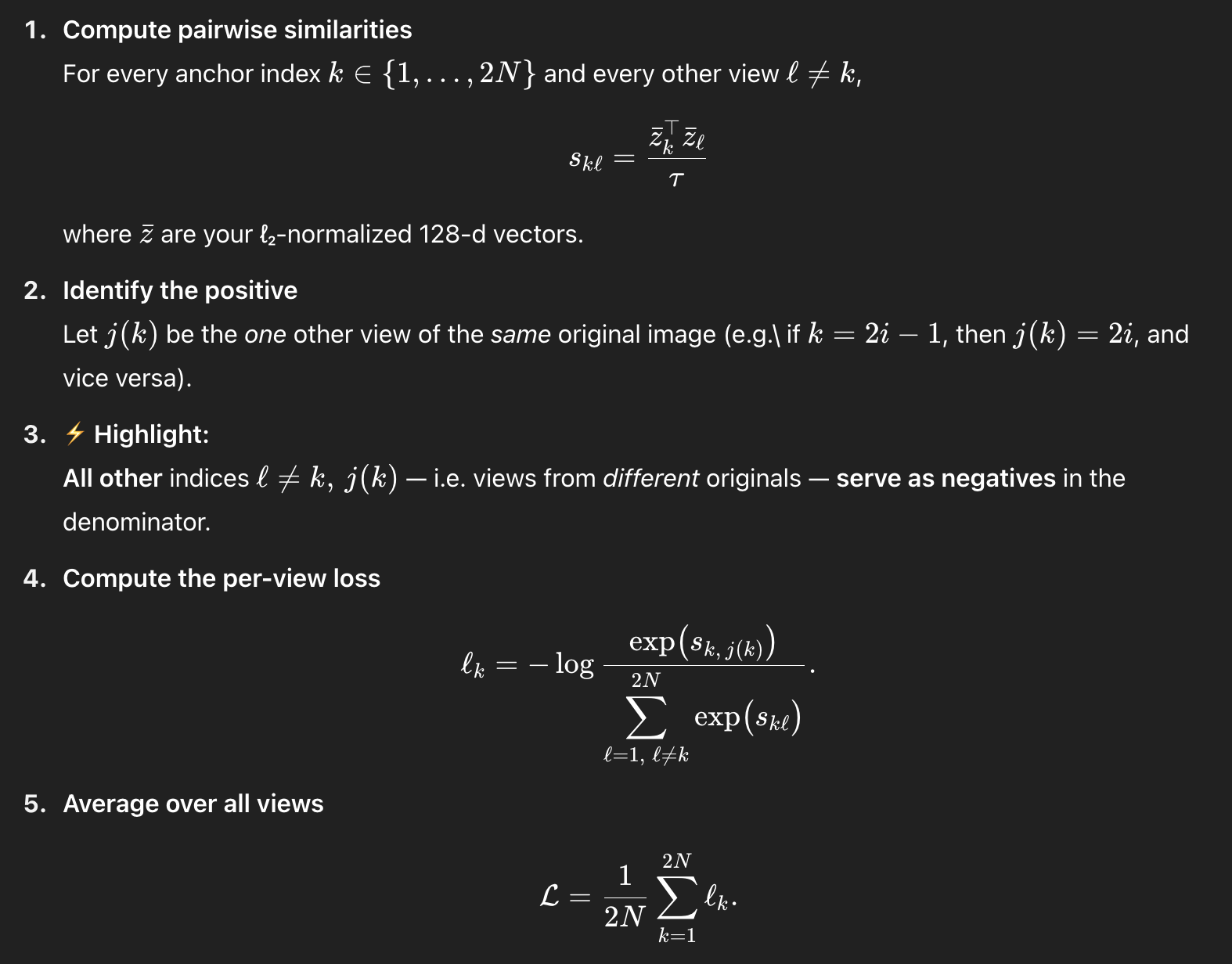
l과 k의 표기에 주의하자. 얘네는 그냥 2N개의 minibatch 속의 인덱스를 뜻하는 것이다. 결국 같은 이미지에서 나온 다른 parameter의 augmentation만 positive pair이고, 나머지는 다 negative pair이다. 이렇게 하면 hard negative mining 같은거 안해도 된다.
Large Batch Size
저자들은 batch size 4096으로 100 epoch 동안 훈련했음을 밝힌다. 이는 8190 negative examples per positive pair from both augmentation views를 준다. 맨 처음에 저자들이 contrastive learning이 성공적이기 위한 조건으로 large batch를 내건 이유는, negative exmaple이 많으면 많을수록 성능이 좋기 때문이다. 아래를 보자.
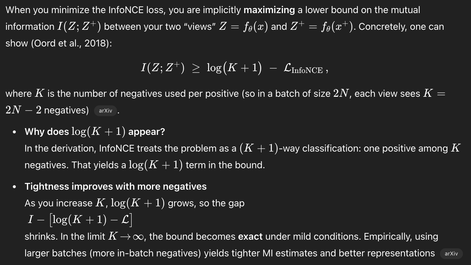
Negative example이 증가하면 할 수록 bound가 tight해지는 효과가 있다고 한다.
자세한 건 아래를 참조.
https://arxiv.org/abs/2005.13149
On Mutual Information in Contrastive Learning for Visual Representations
In recent years, several unsupervised, "contrastive" learning algorithms in vision have been shown to learn representations that perform remarkably well on transfer tasks. We show that this family of algorithms maximizes a lower bound on the mutual informa
arxiv.org
Limitations
당연히 large batch size가 필요하다는 것이 한계점일 수 밖에 없다. 그리고 늘어나는 batch size에 따라 pairwise computation이 진행되기 때문에 quadratically increase하는 computation이 초래되고, high cost of memory가 필요하다. 그래서 gradient accumulation hack이나 memory bank를 대부분 사용한다.
그리고 augmentation과 그 hyperparameter에 결과가 민감하다는 점, 긴 epoch가 필요하다는 점도 있고,
False Negative의 문제도 있다. "하나의" 이미지에서 나온 아이들만 positive pair로 분류하고 나머지는 전부 negative pair로 분류해버리는데, 그러면 여러 장의 사자 이미지가 있어도 비슷하지만 다른 사자 이미지에서 나온 augmented image representation들은 전부 negative example로 분류해버리는 일이 생긴다.
이런 한계점을 극복하기 위해 이후, MoCo’s memory queue, BYOL’s negative‐free design, Debiased Contrastive Learning’s reweighting of false negatives, and distilled or non‐contrastive Siamese methods 가 나온다. 이는 차차 알아보자.